Joining Data

Code for Quiz 6, more dplyr and our first interactive chart using echarts4r.

Steps 1-6

1. Load the R packages we will use.

library(tidyverse)
library(echarts4r)  #install this package before using
library(hrbrthemes)  #install this package before using

2. Read the data in the files, drug_cos.csv, health_cos.csv in to R and assign to the variables drug_cos and health_cos, respectively.

drug_cos  <- read_csv("https://estanny.com/static/week6/drug_cos.csv")
health_cos  <- read_csv("https://estanny.com/static/week6/health_cos.csv")

3. Use glimpse to get a glimpse of the data

drug_cos %>% glimpse()

Rows: 104
Columns: 9
$ ticker       <chr> "ZTS", "ZTS", "ZTS", "ZTS", "ZTS", "ZTS", "Z...
$ name         <chr> "Zoetis Inc", "Zoetis Inc", "Zoetis Inc", "Z...
$ location     <chr> "New Jersey; U.S.A", "New Jersey; U.S.A", "N...
$ ebitdamargin <dbl> 0.149, 0.217, 0.222, 0.238, 0.182, 0.335, 0....
$ grossmargin  <dbl> 0.610, 0.640, 0.634, 0.641, 0.635, 0.659, 0....
$ netmargin    <dbl> 0.058, 0.101, 0.111, 0.122, 0.071, 0.168, 0....
$ ros          <dbl> 0.101, 0.171, 0.176, 0.195, 0.140, 0.286, 0....
$ roe          <dbl> 0.069, 0.113, 0.612, 0.465, 0.285, 0.587, 0....
$ year         <dbl> 2011, 2012, 2013, 2014, 2015, 2016, 2017, 20...

health_cos %>% glimpse()

Rows: 464
Columns: 11
$ ticker      <chr> "ZTS", "ZTS", "ZTS", "ZTS", "ZTS", "ZTS", "ZT...
$ name        <chr> "Zoetis Inc", "Zoetis Inc", "Zoetis Inc", "Zo...
$ revenue     <dbl> 4233000000, 4336000000, 4561000000, 478500000...
$ gp          <dbl> 2581000000, 2773000000, 2892000000, 306800000...
$ rnd         <dbl> 427000000, 409000000, 399000000, 396000000, 3...
$ netincome   <dbl> 245000000, 436000000, 504000000, 583000000, 3...
$ assets      <dbl> 5711000000, 6262000000, 6558000000, 658800000...
$ liabilities <dbl> 1975000000, 2221000000, 5596000000, 525100000...
$ marketcap   <dbl> NA, NA, 16345223371, 21572007994, 23860348635...
$ year        <dbl> 2011, 2012, 2013, 2014, 2015, 2016, 2017, 201...
$ industry    <chr> "Drug Manufacturers - Specialty & Generic", "...

4. Which variables are the same in both data sets

names_drug <- drug_cos %>% names()
names_health <- health_cos %>% names()
intersect(names_drug, names_health)

[1] "ticker" "name"   "year"  

5. Select subset of variables to work with

• For drug_cos select (in this order): ticker, year, grossmargin

  • Extract observations for 2018

  • Assign output to drug_subset

• For health_cos select (in this order): ticker, year, revenue, gp, industry

  • Extract observations for 2018

  • Assign output to health_subset

drug_subset  <- drug_cos  %>% 
  select(ticker, year, grossmargin)  %>% 
  filter(year == 2018)

health_subset  <- health_cos  %>%
  select(ticker, year, revenue, gp, industry)  %>% 
  filter(year == 2018)

6. Keep all the rows and columns drug_subset join with columns in health_subset

drug_subset  %>% left_join(health_subset)

# A tibble: 13 x 6
   ticker  year grossmargin   revenue        gp industry              
   <chr>  <dbl>       <dbl>     <dbl>     <dbl> <chr>                 
 1 ZTS     2018       0.672   5.82e 9   3.91e 9 Drug Manufacturers - ~
 2 PRGO    2018       0.387   4.73e 9   1.83e 9 Drug Manufacturers - ~
 3 PFE     2018       0.79    5.36e10   4.24e10 Drug Manufacturers - ~
 4 MYL     2018       0.35    1.14e10   4.00e 9 Drug Manufacturers - ~
 5 MRK     2018       0.681   4.23e10   2.88e10 Drug Manufacturers - ~
 6 LLY     2018       0.738   2.46e10   1.81e10 Drug Manufacturers - ~
 7 JNJ     2018       0.668   8.16e10   5.45e10 Drug Manufacturers - ~
 8 GILD    2018       0.781   2.21e10   1.73e10 Drug Manufacturers - ~
 9 BMY     2018       0.71    2.26e10   1.60e10 Drug Manufacturers - ~
10 BIIB    2018       0.865   1.35e10   1.16e10 Drug Manufacturers - ~
11 AMGN    2018       0.827   2.37e10   1.96e10 Drug Manufacturers - ~
12 AGN     2018       0.861   1.58e10   1.36e10 Drug Manufacturers - ~
13 ABBV    2018       0.764   3.28e10   2.50e10 Drug Manufacturers - ~

Question: join_ticker

• Start with drug_cos

• Extract observations for the ticker JNJ from drug_cos

• Assign output to the variable drug_cos_subset

drug_cos_subset  <- drug_cos  %>% 
  filter(ticker == "JNJ")

---

• Display drug_cos_subset

drug_cos_subset

# A tibble: 8 x 9
  ticker name  location ebitdamargin grossmargin netmargin   ros   roe
  <chr>  <chr> <chr>           <dbl>       <dbl>     <dbl> <dbl> <dbl>
1 JNJ    John~ New Jer~        0.247       0.687     0.149 0.199 0.161
2 JNJ    John~ New Jer~        0.272       0.678     0.161 0.218 0.173
3 JNJ    John~ New Jer~        0.281       0.687     0.194 0.224 0.197
4 JNJ    John~ New Jer~        0.336       0.694     0.22  0.284 0.217
5 JNJ    John~ New Jer~        0.335       0.693     0.22  0.282 0.219
6 JNJ    John~ New Jer~        0.338       0.697     0.23  0.286 0.229
7 JNJ    John~ New Jer~        0.317       0.667     0.017 0.243 0.019
8 JNJ    John~ New Jer~        0.318       0.668     0.188 0.233 0.244
# ... with 1 more variable: year <dbl>

• Use left_join to combine the rows and columns of drug_cos_subset with the columns of health_cos

• Assign the output to combo_df

combo_df  <- drug_cos_subset  %>% 
  left_join(health_cos)

---

• Display combo_df

combo_df

# A tibble: 8 x 17
  ticker name  location ebitdamargin grossmargin netmargin   ros   roe
  <chr>  <chr> <chr>           <dbl>       <dbl>     <dbl> <dbl> <dbl>
1 JNJ    John~ New Jer~        0.247       0.687     0.149 0.199 0.161
2 JNJ    John~ New Jer~        0.272       0.678     0.161 0.218 0.173
3 JNJ    John~ New Jer~        0.281       0.687     0.194 0.224 0.197
4 JNJ    John~ New Jer~        0.336       0.694     0.22  0.284 0.217
5 JNJ    John~ New Jer~        0.335       0.693     0.22  0.282 0.219
6 JNJ    John~ New Jer~        0.338       0.697     0.23  0.286 0.229
7 JNJ    John~ New Jer~        0.317       0.667     0.017 0.243 0.019
8 JNJ    John~ New Jer~        0.318       0.668     0.188 0.233 0.244
# ... with 9 more variables: year <dbl>, revenue <dbl>, gp <dbl>,
#   rnd <dbl>, netincome <dbl>, assets <dbl>, liabilities <dbl>,
#   marketcap <dbl>, industry <chr>

*Note: the variables ticker, name, location and industry are the same for all the observations

---

• Assign the company name to co_name

co_name  <- combo_df  %>% 
  distinct(name) %>% 
  pull()

---

• Assign the company location to co_location

co_location  <- combo_df  %>% 
  distinct(location)  %>% 
  pull() 

---

• Assign the industry to co_industry group

co_industry  <- combo_df  %>% 
  distinct(industry)  %>% 
  pull()

Put the r inline commands used in the blanks below. When you knit the document the results of the commands will be displayed in your text.

The company Johnson & Johnson is located in New Jersey; USA and is a member of the Drug Manufacturers - General industry group.

---

• Start with combo_df

• Select variables (in this order): year, grossmargin, netmargin, revenue, gp, netincome

• Assign the output to combo_df_subset

combo_df_subset  <- combo_df  %>% 
  select(year, grossmargin, netmargin, revenue, gp, netincome)

---

• Display combo_df_subset

combo_df_subset

# A tibble: 8 x 6
   year grossmargin netmargin     revenue          gp   netincome
  <dbl>       <dbl>     <dbl>       <dbl>       <dbl>       <dbl>
1  2011       0.687     0.149 65030000000 44670000000  9672000000
2  2012       0.678     0.161 67224000000 45566000000 10853000000
3  2013       0.687     0.194 71312000000 48970000000 13831000000
4  2014       0.694     0.22  74331000000 51585000000 16323000000
5  2015       0.693     0.22  70074000000 48538000000 15409000000
6  2016       0.697     0.23  71890000000 50101000000 16540000000
7  2017       0.667     0.017 76450000000 51011000000  1300000000
8  2018       0.668     0.188 81581000000 54490000000 15297000000

---

• Create the variable grossmargin_check to compare with the variable grossmargin. They should be equal.

  • grossmargin_check = gp / revenue

• Create the variable close_enough to check that the absolute value of the difference between grossmargin_check and grossmargin is less than 0.001

combo_df_subset  %>% 
  mutate(grossmargin_check = gp / revenue,
  close_enough = abs(grossmargin_check - grossmargin) < 0.001)

# A tibble: 8 x 8
   year grossmargin netmargin revenue      gp netincome
  <dbl>       <dbl>     <dbl>   <dbl>   <dbl>     <dbl>
1  2011       0.687     0.149 6.50e10 4.47e10   9.67e 9
2  2012       0.678     0.161 6.72e10 4.56e10   1.09e10
3  2013       0.687     0.194 7.13e10 4.90e10   1.38e10
4  2014       0.694     0.22  7.43e10 5.16e10   1.63e10
5  2015       0.693     0.22  7.01e10 4.85e10   1.54e10
6  2016       0.697     0.23  7.19e10 5.01e10   1.65e10
7  2017       0.667     0.017 7.64e10 5.10e10   1.30e 9
8  2018       0.668     0.188 8.16e10 5.45e10   1.53e10
# ... with 2 more variables: grossmargin_check <dbl>,
#   close_enough <lgl>

---

• Create the variable netmargin_check to compare with the variable netmargin. They should be equal.

• Create the variable close_enough to check that the absolute value of the difference between netmargin_check and netmargin is less than 0.001

combo_df_subset  %>% 
  mutate(netmargin_check = netincome / revenue,
  close_enough = abs(netmargin_check - netmargin) < 0.001)

# A tibble: 8 x 8
   year grossmargin netmargin revenue      gp netincome
  <dbl>       <dbl>     <dbl>   <dbl>   <dbl>     <dbl>
1  2011       0.687     0.149 6.50e10 4.47e10   9.67e 9
2  2012       0.678     0.161 6.72e10 4.56e10   1.09e10
3  2013       0.687     0.194 7.13e10 4.90e10   1.38e10
4  2014       0.694     0.22  7.43e10 5.16e10   1.63e10
5  2015       0.693     0.22  7.01e10 4.85e10   1.54e10
6  2016       0.697     0.23  7.19e10 5.01e10   1.65e10
7  2017       0.667     0.017 7.64e10 5.10e10   1.30e 9
8  2018       0.668     0.188 8.16e10 5.45e10   1.53e10
# ... with 2 more variables: netmargin_check <dbl>,
#   close_enough <lgl>

Question: summarize_industry

• Fill in the blanks

• Put the command you use in the Rchunks in the Rmd file for this quiz

• Use the health_cos data

• For each industry calculate

  • mean_grossmargin_percent = mean(gp / revenue) * 100
  • median_grossmargin_percent = median(gp / revenue) * 100
  • min_grossmargin_percent = min(gp / revenue) * 100
  • max_grossmargin_percent = max(gp / revenue) * 100

health_cos  %>% 
  group_by(industry)  %>% 
  summarize(mean_grossmargin_percent = mean(gp / revenue) * 100,
            median_grossmargin_percent = median(gp / revenue) * 100,
            min_grossmargin_percent = min(gp / revenue) * 100,
            max_grossmargin_percent = max(gp / revenue) * 100)

# A tibble: 9 x 5
  industry mean_grossmargi~ median_grossmar~ min_grossmargin~
* <chr>               <dbl>            <dbl>            <dbl>
1 Biotech~             92.5            92.7             81.7 
2 Diagnos~             50.5            52.7             28.0 
3 Drug Ma~             75.4            76.4             36.8 
4 Drug Ma~             47.9            42.6             34.3 
5 Healthc~             20.5            19.6             10.0 
6 Medical~             55.9            37.4             28.1 
7 Medical~             70.8            72.0             53.2 
8 Medical~             10.4             5.38             2.49
9 Medical~             53.9            52.8             40.5 
# ... with 1 more variable: max_grossmargin_percent <dbl>

• mean_grossmargin_percent for the industry Medical Devices is 70.8%

• median_grossmargin_percent for the industry Medical Devices is 72.0%

• min_grossmargin_percent for the industry Medical Devices is 53.2%

• max_grossmargin_percent for the industry Medical Devices is 84.7%

Question: inline_ticker

• Fill in the blanks

• Use the health_cos data

• Extract observations for the ticker AMGN from health_cos and assign to the variable health_cos_subset

health_cos_subset  <- health_cos  %>% 
  filter(ticker == "AMGN")

• Display health_cos_subset

health_cos_subset

# A tibble: 8 x 11
  ticker name  revenue      gp    rnd netincome  assets liabilities
  <chr>  <chr>   <dbl>   <dbl>  <dbl>     <dbl>   <dbl>       <dbl>
1 AMGN   Amge~ 1.56e10 1.29e10 3.17e9    3.68e9 4.89e10 29842000000
2 AMGN   Amge~ 1.73e10 1.41e10 3.38e9    4.34e9 5.43e10 35238000000
3 AMGN   Amge~ 1.87e10 1.53e10 4.08e9    5.08e9 6.61e10 44029000000
4 AMGN   Amge~ 2.01e10 1.56e10 4.30e9    5.16e9 6.90e10 43231000000
5 AMGN   Amge~ 2.17e10 1.74e10 4.07e9    6.94e9 7.14e10 43366000000
6 AMGN   Amge~ 2.30e10 1.88e10 3.84e9    7.72e9 7.76e10 47751000000
7 AMGN   Amge~ 2.28e10 1.88e10 3.56e9    1.98e9 8.00e10 54713000000
8 AMGN   Amge~ 2.37e10 1.96e10 3.74e9    8.39e9 6.64e10 53916000000
# ... with 3 more variables: marketcap <dbl>, year <dbl>,
#   industry <chr>

• In the console, type ?distinct. Go to the help pane to see what distinct does

• In the console, type ?pull. Go to the help pane to see what pull does

Run the code below

health_cos_subset  %>% 
  distinct(name) %>%  
  pull(name)

[1] "Amgen Inc"

• assign the output to co_name

co_name  <- health_cos_subset  %>% 
  distinct(name) %>% 
  pull(name)

You can take output from your code and include it in your text.

• The name of the company with ticker AMGN is Amgen Inc

In following chuck

• Assign the company’s industry group to the variable co_industry

co_industry  <- health_cos_subset  %>% 
  distinct(industry) %>% 
  pull()

This is outside the R chunk. Put the r inline commands used in the blanks below. When you knit the document the results of the commands will be displayed in your text.

The company Amgen Inc is a member of the Drug Manufacturers - General group.

---

Steps 7-11

7. Prepare the data for the plots

• start with health_cos THEN

• group_by industry THEN

• calculate the median research and development expenditure as a percent of revenue by industry

• assign the output to df

df <- health_cos  %>% 
  group_by(industry)  %>%
  summarize(med_rnd_rev = median(rnd/revenue))

8. Use glimpse to glimpse the data for the plots

df  %>% glimpse()

Rows: 9
Columns: 2
$ industry    <chr> "Biotechnology", "Diagnostics & Research", "D...
$ med_rnd_rev <dbl> 0.48317287, 0.05620271, 0.17451442, 0.0685187...

9. Create a static bar chart

• use ggplot to initialize the chart

• data is df

• the variable industry is mapped to the x-axis

  • reorder it based the value of med_rnd_rev

• the variable med_rnd_rev is mapped to the y-axis

• add a bar chart using geom_col

• use scale_y_continuous to label the y-axis with percent

• use coord_flip() to flip the coordinates

• use labs to add title, subtitle and remove x and y-axes

• use theme_ipsum() from the hrbrthemes package to improve the theme

ggplot(data = df, 
       mapping = aes(
         x = reorder(industry, med_rnd_rev ),
         y = med_rnd_rev
         )) +
  geom_col() + 
  scale_y_continuous(labels = scales::percent) +
  coord_flip() +
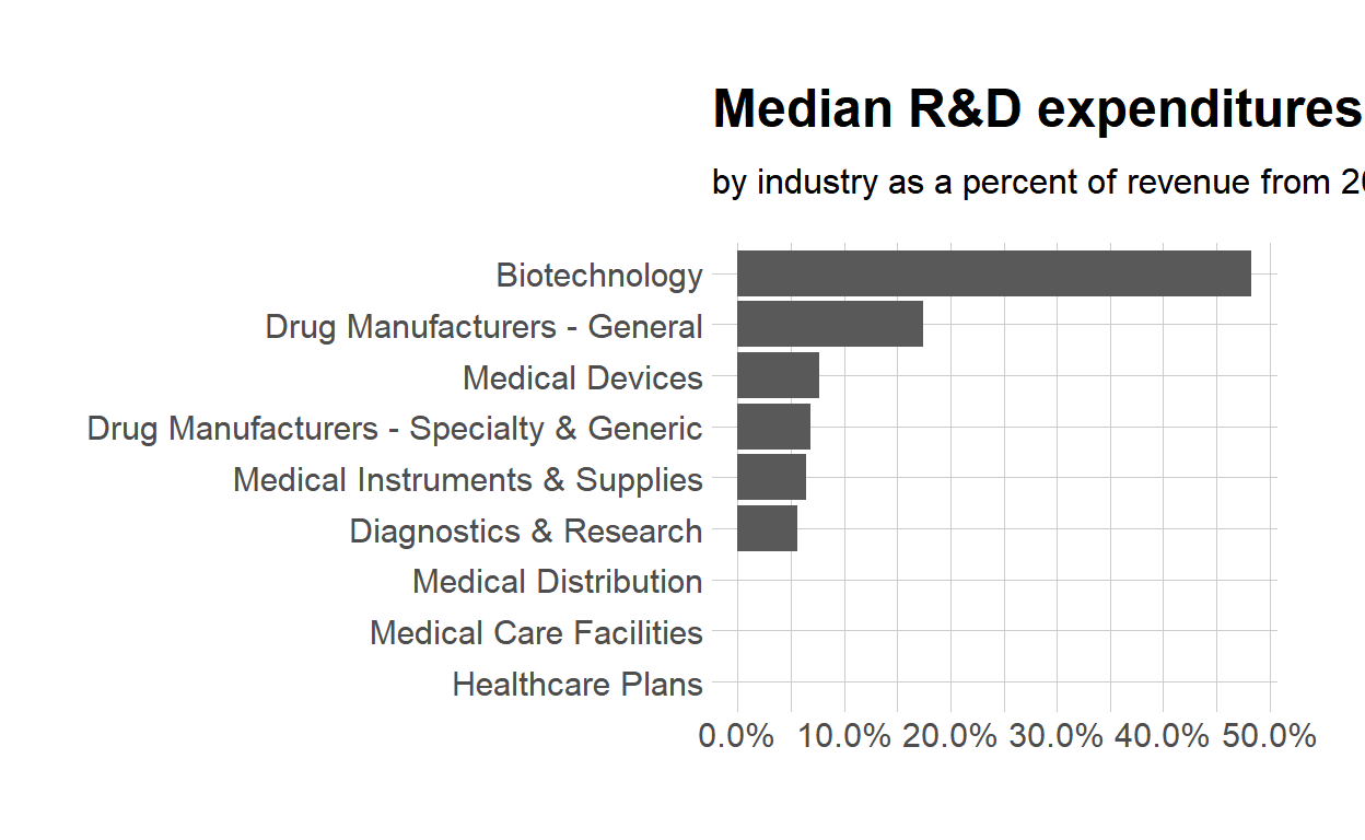
  labs(
    title = "Median R&D expenditures",
    subtitle = "by industry as a percent of revenue from 2011 to 2018",
    x = NULL, y = NULL) +
  theme_ipsum()

10. Save the last plot to preview.png and add to the yaml chunk at the top

ggsave(filename = "preview.png", 
       path = here::here("_posts", "2021-03-11-joining-data"))

11. Create an interactive bar chart using the package echarts4r

• start with the data df

• use arrange to reorder med_rnd_rev

• use e_charts to initialize a chart

  • the variable industry is mapped to the x-axis

• add a bar chart using e_bar with the values of med_rnd_rev

• use e_flip_coords() to flip the coordinates

• use e_title to add the title and the subtitle

• use e_legend to remove the legends

• use e_x_axis to change format of labels on x-axis to percent

• use e_y_axis to remove labels on y-axis-

• use e_theme to change the theme. Find more themes here

df  %>% 
  arrange(med_rnd_rev)  %>%
  e_charts(
    x = industry
    )  %>% 
  e_bar(
    serie = med_rnd_rev, 
    name = "median"
    )  %>%
  e_flip_coords()  %>% 
  e_tooltip()  %>% 
  e_title(
    text = "Median industry R&D expenditures", 
    subtext = "by industry as a percent of revenue from 2011 to 2018",
    left = "center") %>% 
  e_legend(FALSE) %>% 
  e_x_axis(
    formatter = e_axis_formatter("percent", digits = 0)
    )  %>%
  e_y_axis(
    show = FALSE
  )  %>% 
  e_theme("dark")